In-built Aggregate Functions
Aggregate Formula allows you to create powerful metrics to address your business needs. In this section let's learn about the wide range of powerful in-built functions that are supported by Zoho Analytics.
Aggregate Functions
The following table describes these functions:
| Functions | Details |
| Sum | Format: Description: Parameters:
Returns: Example: This calculated the selling price by subtracting the Discount from the Price and then finds the total selling price by adding values for all records. |
| Avg | Format: Description: Parameters:
Returns: Example: This calculated the profit by subtracting the Cost from the Sales for all records and then finds the average of these values. |
| Min | Format: Description: Parameters:
Returns: Example: min("Sales"."Amount") This will find the minimum sales done. Note:
See Also: |
| Max | Format: Description: Parameters:
Returns: Example: max("Sales"."Amount") This will find the maximum sales done. Note:
See Also: |
| Count | Format: Description: Parameters:
Returns: Example: count("Sales"."Customer_ID") This will find the total number of rows with a Customer_ID. Note:
See Also: |
| Distinct Count | Format: Description: Parameters:
Returns: Example: count("Sales"."Customer_ID") This will find the total number of customers present in the data. Note:
See Also: |
| Count_WB | Format: Description: Parameters:
Returns: This returns the count of rows with the expression's result including the null value. Example: count("Feedback"."email_id") This will find the total number of feedback entries with or without the email address. See Also: |
| Stddev | Format: Description: Parameters:
Returns: Example: This returns the standard deviation of the stock price. This helps in measuring the risk involved in the investment. See Also: stddev_samp(), variance(), var_samp() |
| Variance | Format: Description: Parameters:
Returns: Example: This returns the variance of the stock price. This helps in measuring the risk involved in the investment. See Also: stddev_samp(), stddev(), var_samp() |
| SumIf | Format: Description: Parameters:
Returns: Example: This will return the sum of the Amount if the status is not cancelled. Else it will return zero. Note: |
| AvgIf | Format: Description: Parameters:
Returns: Example: This will return the average deal Amount that is lost to Competition. Note: |
| CountIf | Format: Description: Parameters:
Returns: Example: This will return the number of task where the status is overdue. Note: See Also: |
| YTD | Format: Description: Parameters:
Returns: Example: Let's assume that the current date is 17th March 2019. This formula will return the sum of sales for all years till 17th March of that year. |
| QTD | Format: Description: Parameters:
Returns: Example: Let's assume that the current date is 17th March 2019 and you have the calendar year as your fiscal year. This formula will return the sum of sales for all quarters till 17th of the last month of the quarter. |
| MTD | Format: Description: Parameters:
Returns: Example: mtd( sum("Sales"."Sales"),"Sales"."Date") Let's assume that the current date is 17th March 2019. This will return the sum of sales for the all months till the 17th of that month. |
| Mean | Format: Description: Parameters:
Returns: Example: This returns the average deal amount by adding all deal amount and divide it by the number of deals. |
| Median | Format: Description: Parameters:
Returns: Example: This will order the deal amount from least to greatest and return the middle value. |
| Mode | Format: Description: Parameters:
Returns: Example: This will return the Number of Responses taken to close most of the tickets. |
| Percentile | Format: Description: Parameters:
Returns: Example: This will identify a sales value below which 90% of the sales amount lies. |
Groupby Shifting Expressions
By default, Aggregate Formula values will be computed for each data record/group in a report in which it is used. However, to meet your specific requirements, you can also specify how a column's data is to be grouped for computing the values.
The Groupby Shifting Expressions give you more control over how the columns are grouped to compute the values. Zoho Analytics allows you to perform this in the following levels.
- Include Groupby - Adds more columns to a group
- Exclude Groupby - Removes columns to a group
- Fixed Groupby - Sets fixed columns to a group
- Map Groupby - Maps a group by column with another
- Ignore Filters - Ignores the specified user filters being applied on the given aggregate expression.
Include Groupby
The Include Groupby formula allows you to add more dimensions to a group by clause, along with the existing dimensions used, in the report where this Aggregate Formula is used.
Format
Example
In the above expression, we calculate the average of Sales per Customer. The Sum of Sales is first grouped by Customer Name, along with the existing group by columns in the report. This will get the total sales for each customer. Now the average of these values will be displayed in the report i.e., the average of Sales per Customer.
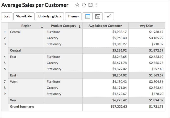
In the above chart, the Avg Sales column shows the total sales average for Product Category in each Region. The aggregate formula Avg Sales per Customer shows the average sales made by a customer.
Exclude Groupby
Exclude Groupby allows you to omit or ignore group by dimensions, that are available in the report when aggregate values are computed.
Format
Example
Here, if the report is grouped by Region, then the above expression will exclude for calculating the sum of Sales.
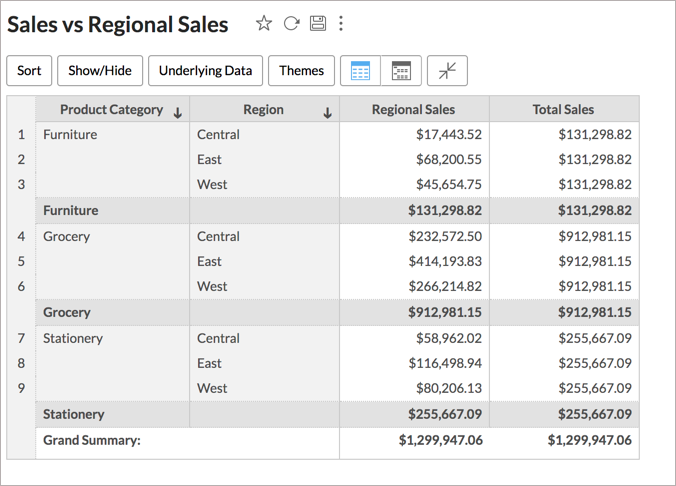
In the above chart, the Regional Sales column shows the total sales in each Region for Product Category. And the aggregate formula shows the total sales in the Product Category ignoring the Region field in the report.
Fixed Groupby
Fixed Groupby allows you to set a specific group by dimensions to compute values, independent of the group by dimensions available in the report.
Format
Example
Here, irrespective of whatever grouping is done in the report, data will be grouped by the absolute quarter of the Date column to compute the sum of Sales. i.e., irrespective of the Regional grouping in the report, the formula will calculate the quarterly sales.
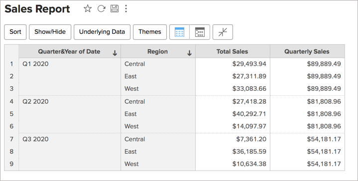
In the above chart, theTotal Sales shows the sales for the dimension in the chart. The aggregate formula Quarterly Sales shows the sales in each quarter irrespective of the dimension used in the report.
Map Groupby
This Map Groupby maps a group by column with another. When you use the first group by column in the report, the aggregate expression will be calculated based on the mapped column instead of the column in the report.
Format
Example
In the above expression, when you add Order Date as a dimension in your report, the sum of delivered sales will be calculated based on the Delivery Date instead of Order Date.
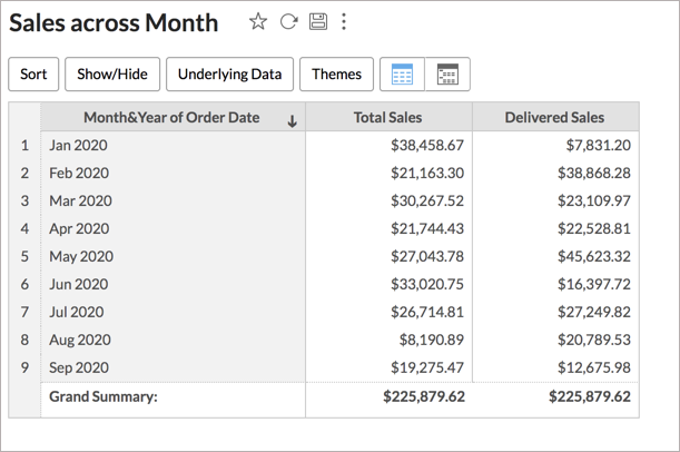
In the above chart, the total sales gets the sales amount for all orders received based on Order Date and Delivered sales gets the sales amount for delivered orders based on delivered date.
Ignore Filters
The Ignore Filters function allows you to ignore the filters applied on the report based on the specified column while calculating the aggregate expression.
Format
You can specify the Filter Type using the following options.
- 0 - This ignores the User Filters applied over the report.
- 1 - This ignores the Filters applied over the report.
- 2 - This ignores both the User Filters and the Filters applied over the report.
If Filter Type is not specified, 0 will be taken as the default value and ignores the User Filters applied over the report.
Example 1
The above expression will return the sum of sales. Filter Type is not specified here, so 0 will be taken as the default value. User Filters based on the Region column will be ignored.
Example 1
The above expression will return the sum of sales. Filters and User Filters based on the Region column will be ignored.
Tabular Functions
The Tabular Function enables you to perform an aggregate calculation across a set of rows that are related to the current row. Unlike in aggregate functions where the query groups the result into a single output row, a tabular function accesses more than just the current row of the query result, allowing you to perform advanced operations.
The following table describes the Tabular functions:
| Functions | Details |
| Window_Sum | Format: Description:& Parameters:
You can also use variables to define the start and end values of the partition window. Returns: Example 1: This calculates the sum of sales for each row, then the result of the current row will be summed with the result of 1 Preceding row and 2 Succeeding rows, within the partition. Example 2: window_sum(sum("Sales"."Sales"),1, ${Variable}) When the variable value is 2, it calculates the sum of sales of each row, then the result of the current row will be summed with the result of 1 preceding row and 2 succeeding rows.
See Also: |
| Window_Average | Format: Window_Avg(AggExpr, Start, End) Description: The Window_Average function finds the average of all the results of the aggregate expressions within the partition. By default, the full frame will be considered as the partition. Parameters:
Returns: This function returns the average value of the results of the aggregate expression (aggexpr). Example: This calculates the sum of sales for each row. Then it will find the average among the result of the current row, along with 2 Preceding rows, and 2 Succeeding rows, within the partition. See Also: |
| Window_Count | Format: window_count(AggExpr, Start, End) Description: The Window_Count function finds the count of the result of the aggregate expression within the partition. Parameters:
Returns: Example: This will return the number of sales records within the partition. See Also: |
| Window_Minimum | Format: window_min(AggExpr, Start, End) Description: The Window_Minimum function finds the minimum value of the result of the aggregate expression within the partition. Parameters:
Returns: This returns the minimum value among the results of the aggregate expression (aggexpr). Example: window_min(sum("Sales"."Sales")) This will calculate the sum of sales and returns the minimum sales within the partition for all rows. See Also: |
| Window_Maximum | Format: Window_Max(AggExpr, Start, End) Description: The Window_Maximum function finds the maximum value of the result of the aggregate expression within the partition. Parameters:
Returns: This returns the maximum value of the results of the aggregate expression (aggexpr). Example: window_max(sum("Sales"."Sales")) This will calculate the sum of sales and returns the maximum sales within the partition for all rows. See Also: Window_Min(), Window_Avg(), Window_Count() |
| Windows_STD | Format: Windows_STD(AggExpr, Start, End) Description: The Windows_STD function finds the standard deviation based on the result of the aggregate expression within the partition. By default full frame will be considered as the partition. Parameters:
Returns: This returns the standard deviation for the results of the aggregate expression (aggexpr). Example: Window_STD(Sum("Sales"."Sales")) This will return the standard deviation based on the sum of sales for all rows within the partition. |
| Windows_Variance | Format: Windows_Variance(AggExpr, Start, End) Description: The Windows_Variance function finds the Variance based on the result of the aggregate expression within the partition. By default full frame will be considered as the partition. Parameters:
Returns: This returns the variance for the results of the aggregate expression (aggexpr). Example: window_variance(sum("Sales"."Sales")) This will return the Variance based on the sum of sales for all rows within the partition. |
| Running Sum | Format: running_sum(AggExpr) Description: The Running Sum will add the result of the aggregate function from the first row in the partition to the current row. Parameters:
Returns: This return the running sum for the results of the aggregate expression (aggexpr). Example: running_sum(sum("Sales"."Sales")) This will return the running sum of sales for all rows within the partition. See Also: Window_Sum(), Running_Sum(), Running_Avg(), Running_Count() |
| Running Average | Format: running_avg(AggExpr) Description: The function gets the running average based on the result of the aggregate function, from the first row in the partition to the current row. Parameters:
Returns: This returns the running average for the results of the aggregate expression (aggexpr). Example: running_avg(sum("Sales"."Sales")) This will return the running average based on the sum of sales for all rows within the partition. See Also: Window_Avg(), Window_Count(), Running_Sum() |
| Running_Count | Format: Running_Count(AggExpr) Description: The function gets the running count based on the result of the aggregate function, from the first row in the partition to the current row. Parameters:
Returns: This returns the running count for the results of the aggregate expression (aggexpr). Example: running_count(sum("Sales"."Sales")) This will return the running count of sales for all rows within the partition. See Also: Window_Count(), Running_Sum(), Running_Avg() |
| Running_Maximum | Format: Running_Max(AggExpr) Description: The function gets the running maximum based on the result of the aggregate function, from the first row in the partition to the current row. Parameters:
Returns: This returns the running maximum for the results of the aggregate expression (aggexpr). Example: running_max(sum("Sales"."Sales")) This will return the running maximum based on sum of sales for all rows within the partition. See Also: Running_Sum(), Running_Avg(), Running_Count, Running_Min() |
| Running_Minimum | Format: Running_Min(AggExpr) Description: The function gets the running minimum based on the result of the aggregate function, from the first row in the partition to the current row. Parameters:
Returns: This returns the running minimum for the results of the aggregate expression (aggexpr). Example: running_min(sum("Sales"."Sales")) This will return the running minimum based on sum of sales for all rows within the partition. See Also: Running_Sum(), Running_Avg(), Running_Count, Running_Max() |
| Rank | Format: Rank(AggExpr, asc/desc) Description: The function gets standard competition ranking for the result of the aggregate expression. Parameters:
Returns: This returns the standard competition ranking based on the results of the aggregate expression (aggexpr). Example: rank(count("Sales"."Sales")) This will return the ranking based on the sum of sales. |
| Dense Rank | Format: dense_rank(AggExpr, start, end) Description: The function gets dense rank for the result of the aggregate expression. Parameters:
Returns: This returns the dense rank for results of the aggregate expression (aggexpr). Example: dense_rank(count("Sales"."Sales")) This will return the dense ranking based on the sum of sales. i.e., in case two values takes the same rank, then the next value will will skip a rank Like 1, 2, 2, 4. |
| Percent_Rank | Format: percent_rank(AggExpr, start, end) Description: The Percent_Rank gets ranking in percent for the result of the aggregate expression. Parameters:
Returns: This returns the ranking in percent for results of the aggregate expression (aggexpr). Example: rank(count("Sales"."Sales")) This will return the ranking in percent based on the sum of sales. i.e., 0.34, 0.36, ... |
| Cume_Dist | Format: cume_dist(AggExpr, asc/desc) Description: The function gets cumulative distribution for the result of the aggregate expression. Parameters:
Returns: This returns the cumulative distribution for results of the aggregate expression (aggexpr). Example: cume_dist(sum("Sales"."Sales")) This returns the cumulative distribution for sum of sales in descending order. |
| Row_Number | Format: row_number(AggExpr) Description: The Row_Number function gets a sequential row number for the result of the aggregate expression. Parameters:
Returns: This returns the row number for results of the aggregate expression (aggexpr). Example: row_number(sum("Sales"."Sales")) This adds row number for all the rows. |
First
| Format: First(AggExpr) Description: The First function gets the result of the aggregate expression for the first row within the partition. Parameters:
Returns: This returns the result of the aggregate expression (aggexpr) for the first row to all rows. Example: first(sum("Sales"."Sales")) This gets the sum of sales for the first row as the result for all rows. |
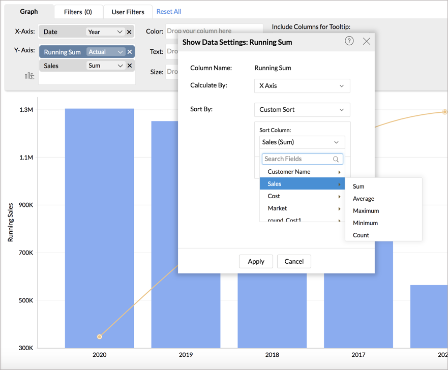
Data Settings
Zoho Analytics allows you to change the partition or sorting order to apply the calculation in the report as needed. Click the Aggregate Formula dropped in the report, the Show Data Setting:{Column Name} dialog will open. The result will be computed based on the setting here.
Calculate By
The Calculate By field allows you to specify the column based on which the calculation needs to be calculated.
For example, the following report shows the running total of sales by region across the months.
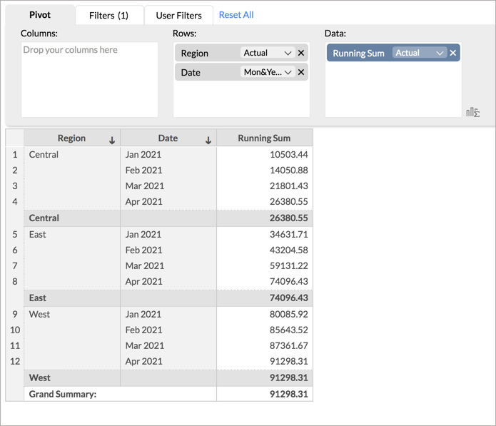
By default, the running sales will be calculated for all the rows in the report. Hence in the above chart, the running sum of the Central will be added to the East values. To calculate the running total for each region across the months, follow the below steps.
- In the Calculate By field, select By Base Fields.
- All the rows in the report will be listed. Select the column based on which you want to calculate the Running Sum. Here, we select Date (Month&Year).
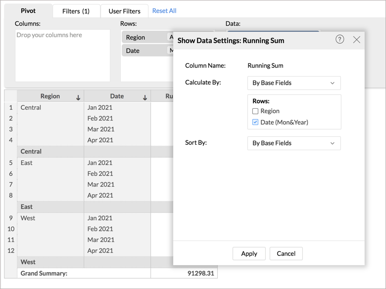
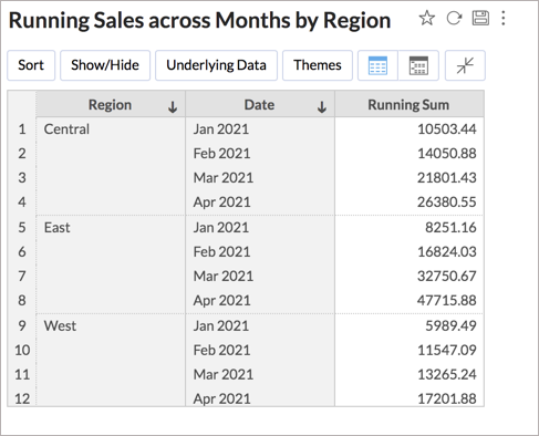
- Click Apply. The running total will be computed across the months for each region.


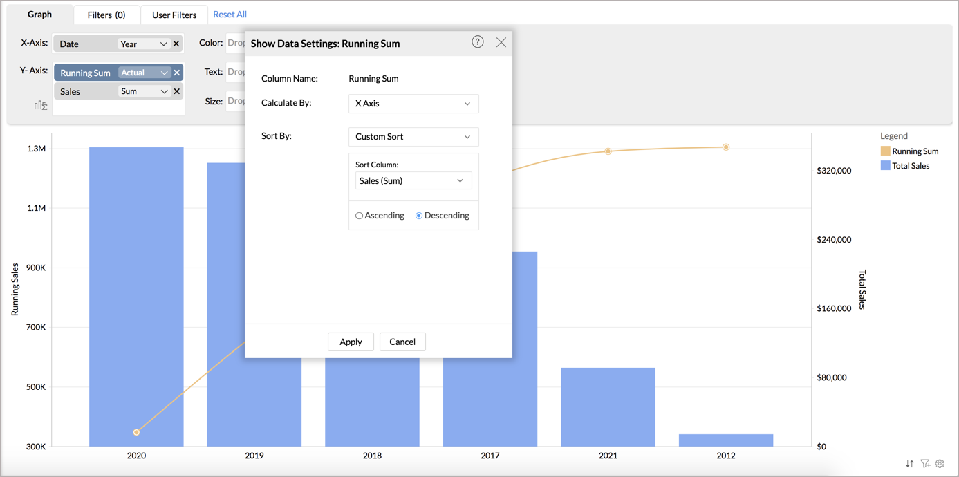
Sort By
Using the Sort By option, you can choose to sort the rows in the report based on any column in the table over which the report is created. The calculation will be performed based on this order.
For example, in the below chart, the running total is sorted based on another metric in the table i.e., sum of sales.
Solutions
Moving Calculation with Dynamic Window
Moving Calculations are ideal for analyzing data sets that fluctuate a lot. Be it stock prices, temperature, or daily sales trend, moving calculation allows you to identify the trend. It smoothens the noise of the random short-term fluctuations from your report.